Visualization

library(tidyverse)
library(ggplot2)
library(plotly)

theme_set(theme_minimal() + theme(legend.position = "bottom"))

options(
  ggplot2.continuous.colour = "viridis",
  ggplot2.continuous.fill = "viridis"
)

scale_colour_discrete = scale_colour_viridis_d
scale_fill_discrete = scale_fill_viridis_d

select <- dplyr::select

happ_df = read_csv("Data/happiness.csv")

Life Ladder Scores Based on Different Regions

Overall mean life ladder score

We want to first get a general sense about the differences among life ladder scores for different regions by plotting the mean life ladder score for each region throughout the years.

happ_df %>%
  group_by(regional_indicator) %>%
  summarise(mean_ladder_score = mean(ladder_score)) %>%
  mutate(regional_indicator = fct_reorder(regional_indicator, mean_ladder_score, .desc = TRUE)) %>%
  ggplot(aes(x = regional_indicator, y = mean_ladder_score, fill = regional_indicator)) +
  geom_bar(stat = "identity", show.legend = FALSE) +
  coord_flip() +
  labs(
    y = "Mean life ladder score",
    x = "Region",
    title = "Mean Life Ladder Score for Different Regions"
  )

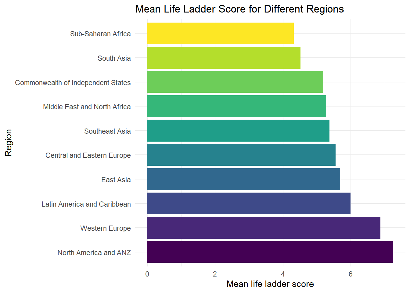
From the years 2005 to 2021, North America and ANZ region has the highest mean life ladder score. Western Europe region has the second highest mean ladder score and is close to North America and ANZ’s. Sub-Saharan Africa and South Asia have the two lowest mean life ladder scores in which Sub-Saharan Africa has the lowest mean life ladder score.

Across Years 2005 to 2021

After getting an idea of the differences of mean life ladder score among different regions, we want to explore the distribution of life ladder score on each region across the years.

happ_df %>%
  filter(year != 2005) %>%
  ggplot(aes(x = year, y = ladder_score, group = year)) +
  geom_boxplot() +
  theme(
    axis.text.x = element_text(angle = 60, vjust = 0.5, hjust = 1, margin = margin(-10, 0, 0, 0)),
    axis.title.x = element_text(margin = margin(15, 0, 0, 0))
  ) +
  facet_wrap(~regional_indicator, nrow = 2) +
  labs(
    x = "Year",
    y = "Life ladder score",
    title = "Life Ladder Scores for Different Regions Across Years"
  )

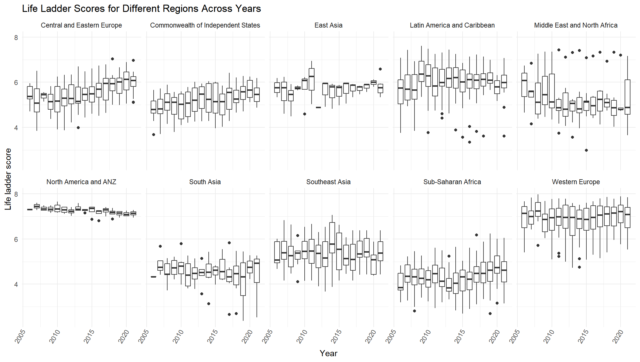
With the initial idea that the mean life ladder score of the North America and ANZ region being the highest, we can see that each year the life ladder score of the North America and ANZ region has similar distribution around 7. For Sub-Saharan Africa, it also has similar distribution in life ladder score around 4 across the years. It seems that the Middle East and North Africa region has many outliers in each year’s life ladder score.

Mean life ladder score for top 50 countries

Now we want to look at the countries that have top 50 mean life ladder score and which regions they belong to.

happ_df %>%
  group_by(country_name, regional_indicator) %>%
  summarise(mean = mean(ladder_score)) %>%
  ungroup() %>%
  top_n(50, mean) %>%
  mutate(country_name = fct_reorder(country_name, mean)) %>%
  ggplot(aes(x = country_name, y = mean, color = regional_indicator)) +
  geom_point(stat = "identity") +
  theme(axis.text.x = element_text(angle = 60, vjust = 1, hjust = 1),
        legend.position = "top") +
  labs(
    x = "Country",
    y = "Mean life ladder score",
    color = "Region"
  )

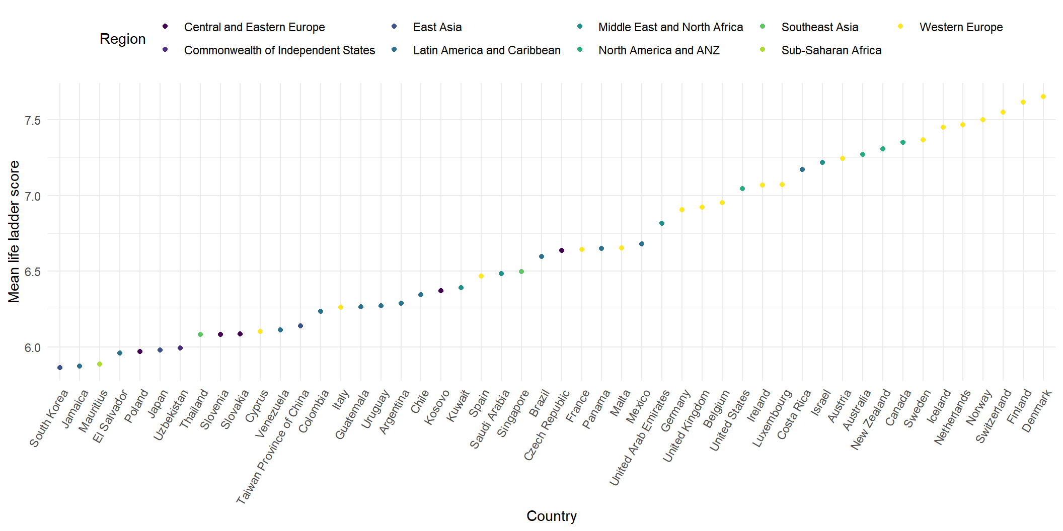
Interestingly, there are many countries from Western Europe and they also have relatively high mean life ladder score across the years.

Other variables Based on Different Regions

Now we want to look at the other variables other than Life Ladder Score since we are interested in exploring the possible factors contributing to happiness.

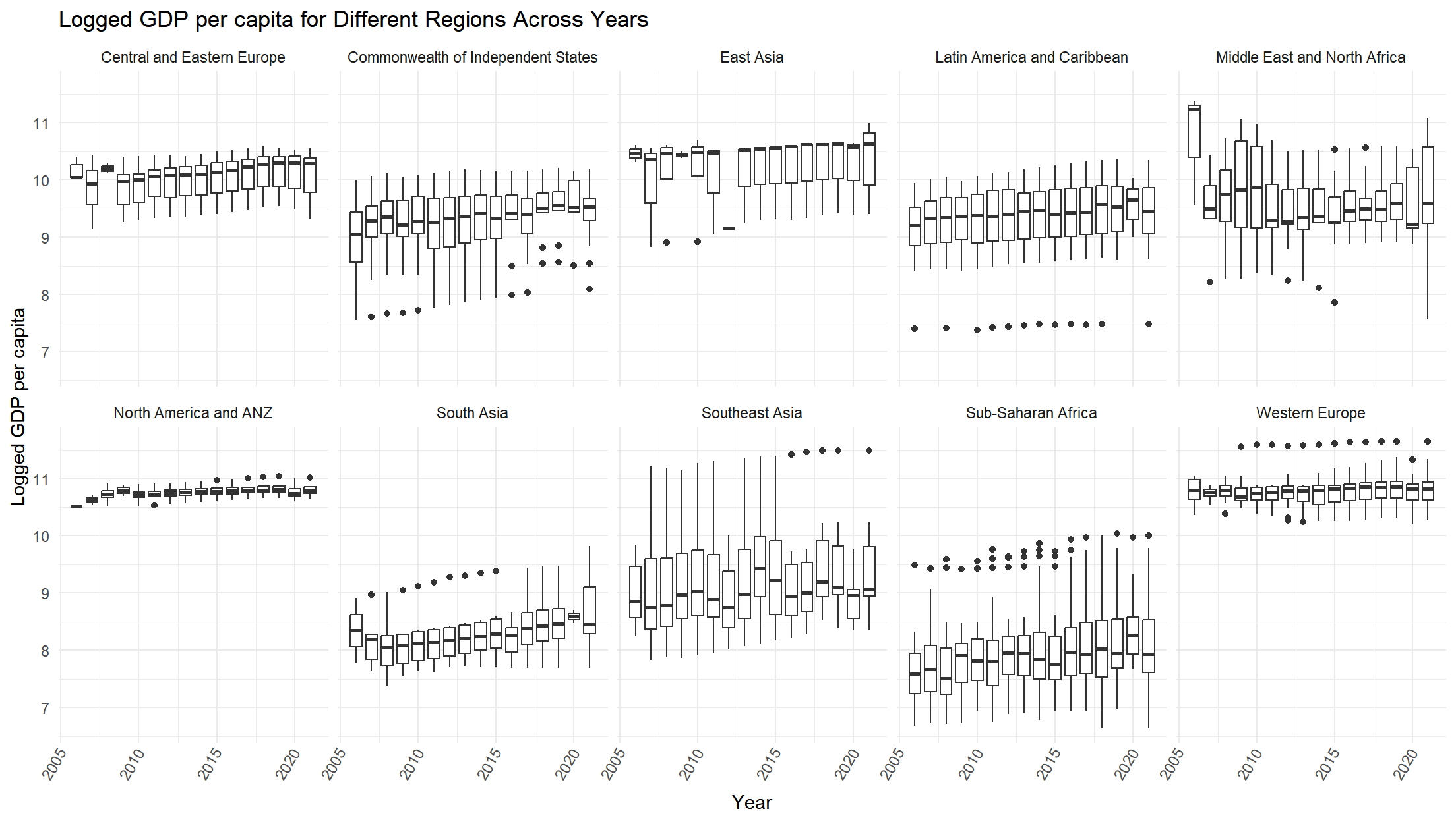
Logged GDP per capita

We can see that the distributions in North America and ANZ, and Western Europe are similar in logged GDP per capita and they are the two highest among these regions. Expectedly, the distribution of Sub-Saharan Africa region is the lowest on the GDP scale.

happ_df %>%
  filter(year != 2005) %>%
  ggplot(aes(x = year, y = logged_gdp_per_capita, group = year)) +
  geom_boxplot() +
  theme(
    axis.text.x = element_text(angle = 60, vjust = 0.5, hjust = 1, margin = margin(-10, 0, 0, 0)),
    axis.title.x = element_text(margin = margin(15, 0, 0, 0))
  ) +
  facet_wrap(~regional_indicator, nrow = 2) +
  labs(
    x = "Year",
    y = "Logged GDP per capita",
    title = "Logged GDP per capita for Different Regions Across Years"
  )

Social support

Western Europe and North America and ANZ regions have similar distribution and the overall positions are the two highest on the social support scale. Surprisingly, the Sub-Saharan Africa region is not the lowest one on this scale, but has many outliers and larger range.

happ_df %>%
  filter(year != 2005) %>%
  ggplot(aes(x = year, y = social_support, group = year)) +
  geom_boxplot() +
  theme(
    axis.text.x = element_text(angle = 60, vjust = 0.5, hjust = 1, margin = margin(-10, 0, 0, 0)),
    axis.title.x = element_text(margin = margin(15, 0, 0, 0))
  ) +
  facet_wrap(~regional_indicator, nrow = 2) +
  labs(
    x = "Year",
    y = "Social support",
    title = "Social Support for Different Regions Across Years"
  )

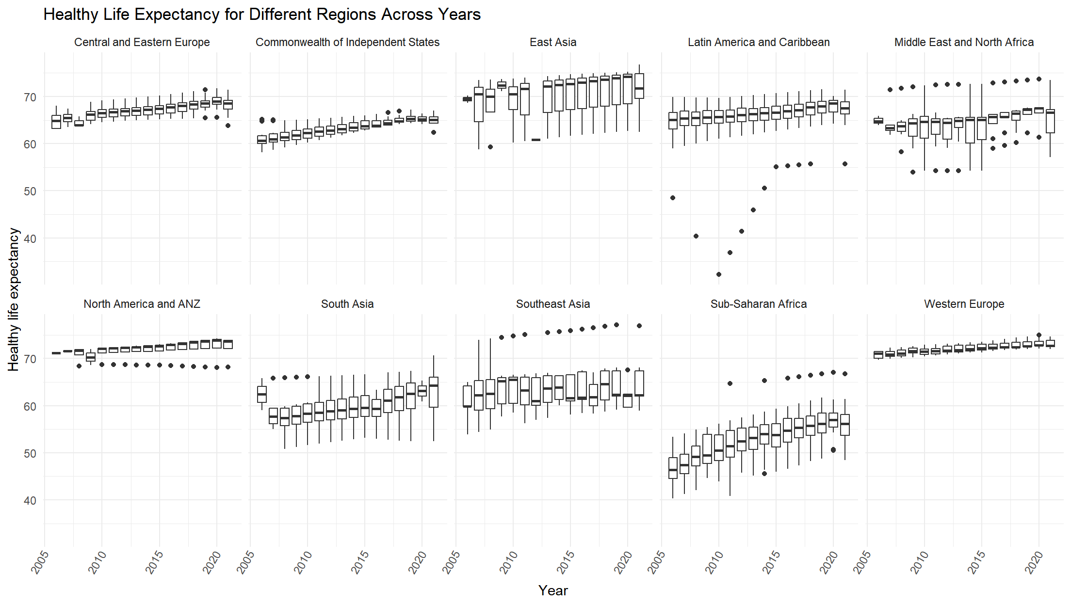
Healthy life expectancy

The regions of Western Europe and North America and ANZ again are the two highest on the scale; Sub-Saharan Africa being the lowest.

happ_df %>%
  filter(year != 2005) %>%
  ggplot(aes(x = year, y = healthy_life_expectancy, group = year)) +
  geom_boxplot() +
  theme(
    axis.text.x = element_text(angle = 60, vjust = 0.5, hjust = 1, margin = margin(-10, 0, 0, 0)),
    axis.title.x = element_text(margin = margin(15, 0, 0, 0))
  ) +
  facet_wrap(~regional_indicator, nrow = 2) +
  labs(
    x = "Year",
    y = "Healthy life expectancy",
    title = "Healthy Life Expectancy for Different Regions Across Years"
  )

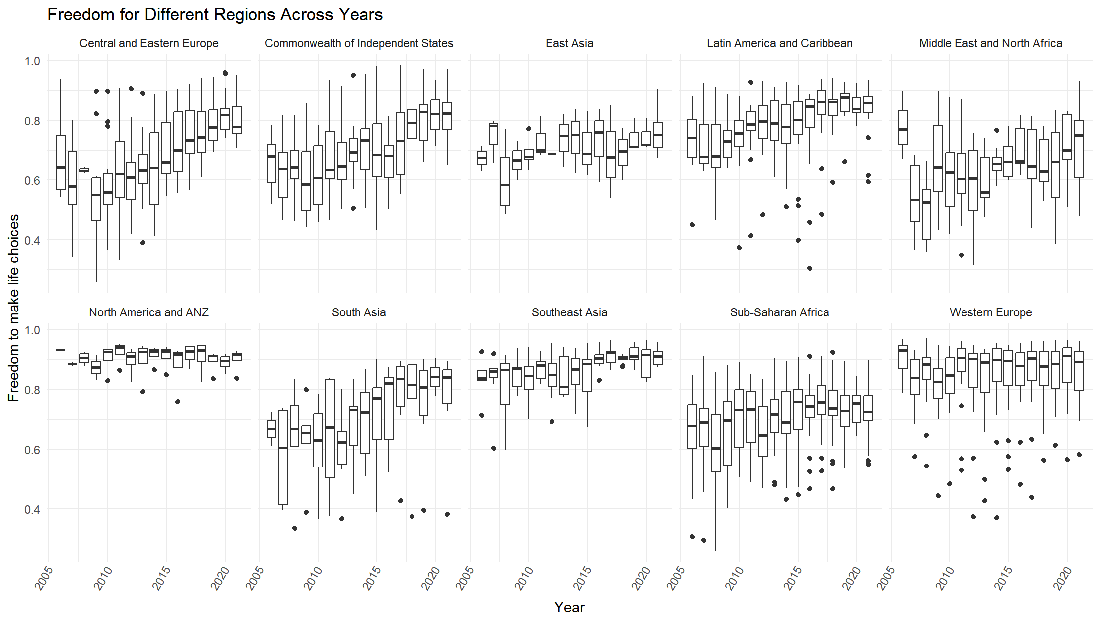
Freedom to make life chocies

This time the distribution does not follow the previous trend. It seems that as time moves on, people in most regions are more satisfied with their freedom to choose what they do with their lives.

happ_df %>%
  filter(year != 2005) %>%
  ggplot(aes(x = year, y = freedom_to_make_life_choices, group = year)) +
  geom_boxplot() +
  theme(
    axis.text.x = element_text(angle = 60, vjust = 0.5, hjust = 1, margin = margin(-10, 0, 0, 0)),
    axis.title.x = element_text(margin = margin(15, 0, 0, 0))
  ) +
  facet_wrap(~regional_indicator, nrow = 2) +
  labs(
    x = "Year",
    y = "Freedom to make life choices",
    title = "Freedom for Different Regions Across Years"
  )

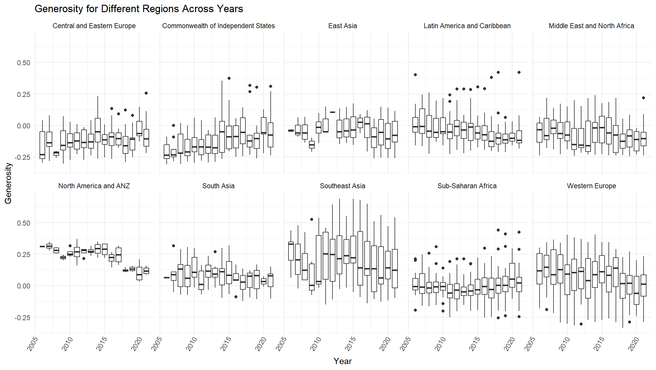
Generosity

For North America and ANZ, Western Europe, and Latin America and Caribbean regions, we can see that the generosity trend is likely to decrease across the years. The rest of the regions do not show an obvious trend in distribution.

happ_df %>%
  filter(year != 2005) %>%
  ggplot(aes(x = year, y = generosity, group = year)) +
  geom_boxplot() +
  theme(
    axis.text.x = element_text(angle = 60, vjust = 0.5, hjust = 1, margin = margin(-10, 0, 0, 0)),
    axis.title.x = element_text(margin = margin(15, 0, 0, 0))
  ) +
  facet_wrap(~regional_indicator, nrow = 2) +
  labs(
    x = "Year",
    y = "Generosity",
    title = "Generosity for Different Regions Across Years"
  )

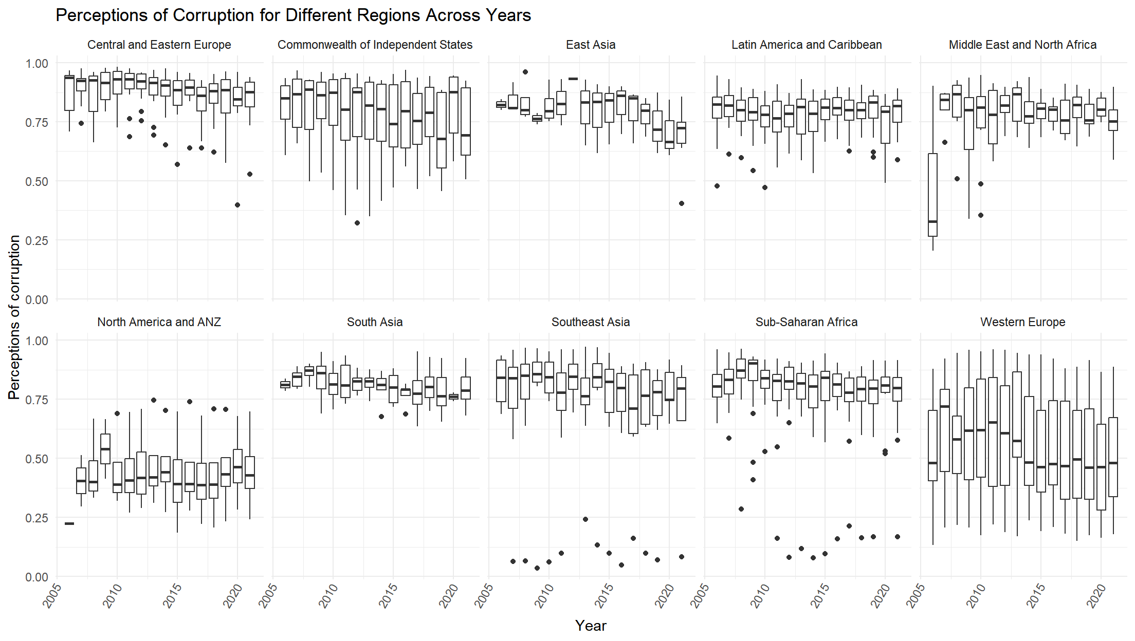
Perceptions of corruption

Surprisingly, only North America and ANZ region is obviously the lowest on the scale. The range of each year’s distribution in Western Europe is large. It seems that the rest of the regions generally think there is corruption widespread throughout the government/businesses.

happ_df %>%
  filter(year != 2005) %>%
  ggplot(aes(x = year, y = perceptions_of_corruption, group = year)) +
  geom_boxplot() +
  theme(
    axis.text.x = element_text(angle = 60, vjust = 0.5, hjust = 1, margin = margin(-10, 0, 0, 0)),
    axis.title.x = element_text(margin = margin(15, 0, 0, 0))
  ) +
  facet_wrap(~regional_indicator, nrow = 2) +
  labs(
    x = "Year",
    y = "Perceptions of corruption",
    title = "Perceptions of Corruption for Different Regions Across Years"
  )

Global Maps

The global maps show the mean values of each variable for the countries with the corresponding color density. White regions are countries without data from that variable.

iso_code <- 
  read.csv("https://raw.githubusercontent.com/plotly/datasets/master/2014_world_gdp_with_codes.csv") %>%
  janitor::clean_names() %>%
  rename(country_name = country) %>%
  select(-gdp_billions) %>%
  add_row(country_name = "Palestinian Territories", code = "PSE")

happy <- 
  read_csv('Data/happiness.csv') %>%
  filter(year != 2005) %>%
  group_by(country_name) %>%
  summarise(mean_ladder_score = mean(ladder_score),
            mean_gdp = mean(logged_gdp_per_capita),
            mean_social_support = mean(social_support),
            mean_expectancy = mean(healthy_life_expectancy),
            mean_freedom = mean(freedom_to_make_life_choices),
            mean_generosity = mean(generosity),
            mean_corruption = mean(perceptions_of_corruption))

happy_name <- unique(happy$country_name)
name <- unique(iso_code$country_name)
diff_name <- setdiff(happy_name,name)
code_name <- c("Congo, Republic of the","Gambia, The", "Hong Kong", "Cote d'Ivoire" ,"Burma", "Cyprus", "Macedonia", "Korea, South", "Taiwan")

for (i in 1:length(code_name)) {
  iso_code$country_name[iso_code$country_name == code_name[i]] <- diff_name[i]
}

happy <- left_join(happy,iso_code)

g <- list(
  showframe = FALSE,
  projection = list(type = 'Mercator')
)

Life Ladder Score

plot_ly(
  happy, 
  type = 'choropleth', 
  locations = happy$code, 
  z = happy$mean_ladder_score, 
  text = happy$country_name, 
  colors = 'Blues'
  ) %>% 
  layout(
    title = "Global Life Ladder Score",
    geo = g
  )